# Initial packages required (we'll be adding more)
library(tidyverse)
library(datasets)
library(fec16)
library(ggplot2)
library(tidycensus)
library(dplyr)
library(sf)
library(ggspatial)
library(mdsr) # package associated with our MDSR bookMaps
library(maps)
us_states <- map_data("state")
head(us_states)
long lat group order region subregion
1 -87.46201 30.38968 1 1 alabama <NA>
2 -87.48493 30.37249 1 2 alabama <NA>
3 -87.52503 30.37249 1 3 alabama <NA>
4 -87.53076 30.33239 1 4 alabama <NA>
5 -87.57087 30.32665 1 5 alabama <NA>
6 -87.58806 30.32665 1 6 alabama <NA>StatePopulation <- read.csv("https://raw.githubusercontent.com/ds4stats/r-tutorials/master/intro-maps/data/StatePopulation.csv", as.is = TRUE)us_rent_income |>
filter(variable == "income") |>
mutate(name = str_to_lower(NAME)) |>
select(-NAME) |>
right_join(us_states, by = c("name" = "region")) |>
ggplot(mapping = aes(x = long, y = lat,
group = group)) +
geom_polygon(aes(fill = estimate), color = "black") +
labs(title = "Average 2017 Income by State", fill = "Yearly Income (in USD)") +
coord_map() +
theme_mdsr()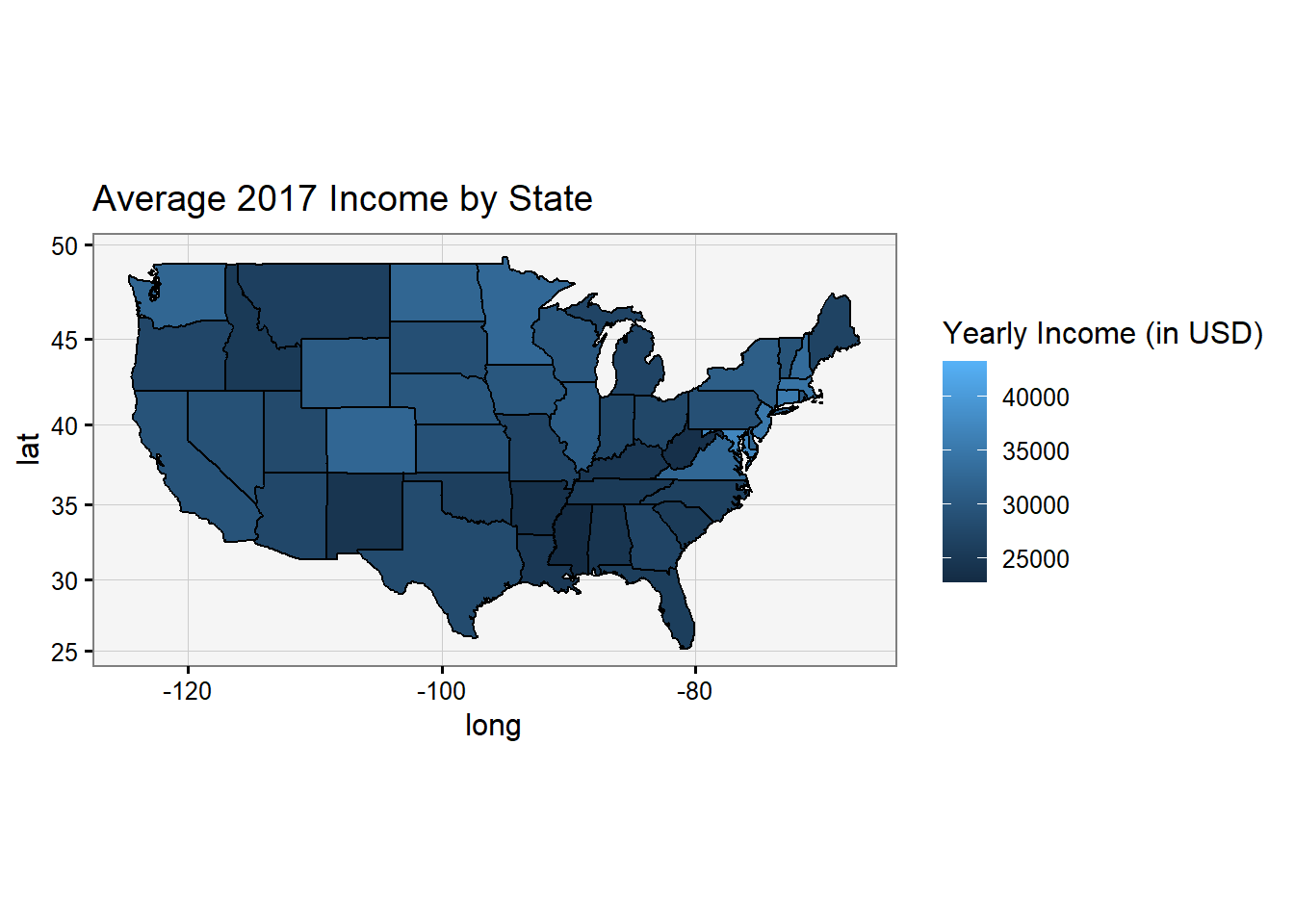
We can see that states like Maryland and Washington had a greater yearly income for 2017 while states like Alabama and West Virginia were not as fortuitous. It’s interesting how states like Maryland and Virginia are doing well while their neighbors are all on the other end of the spectrum. One other thing to note is that the Southeast US tended to earn less than most other regions.
# summary of the 8 congressional Wisconsin districts and the 2016 voting
district_elections <- results_house |>
  mutate(district = parse_number(district_id)) |>
  group_by(state, district) |>
  summarize(
    N = n(),
    total_votes = sum(general_votes, na.rm = TRUE),
    d_votes = sum(ifelse(party == "DEM", general_votes, 0), na.rm = TRUE),
    #we add together all the votes for democrats in the district
    r_votes = sum(ifelse(party == "REP", general_votes, 0), na.rm = TRUE),
    #same but with only republicans
    .groups = "drop"
  ) |>
  mutate(
    other_votes = total_votes - d_votes - r_votes,
    r_prop = r_votes / total_votes,
    winner = ifelse(r_votes > d_votes, "Republican", "Democrat")
  )

wi_results <- district_elections |>
  filter(state == "WI")
wi_results |>
  select(-state)
# A tibble: 8 × 8
district N total_votes d_votes r_votes other_votes r_prop winner
<dbl> <int> <dbl> <dbl> <dbl> <dbl> <dbl> <chr>
1 1 7 353990 107003 230072 16915 0.650 Republican
2 2 2 397581 273537 124044 0 0.312 Democrat
3 3 2 257401 257401 0 0 0 Democrat
4 4 4 285858 220181 0 65677 0 Democrat
5 5 3 390507 114477 260706 15324 0.668 Republican
6 6 4 356935 133072 204147 19716 0.572 Republican
7 7 4 362061 138643 223418 0 0.617 Republican
8 8 4 363574 135682 227892 0 0.627 Republican# Download congressional district shapefiles
options(timeout = 200)
src <- "http://cdmaps.polisci.ucla.edu/shp/districts113.zip"
lcl_zip <- fs::path(tempdir(), "districts113.zip")
download.file(src, destfile = lcl_zip)
lcl_districts <- fs::path(tempdir(), "districts113")
unzip(lcl_zip, exdir = lcl_districts)
dsn_districts <- fs::path(lcl_districts, "districtShapes")
# read shapefiles into R as an sf object
st_layers(dsn_districts)Driver: ESRI Shapefile
Available layers:
layer_name geometry_type features fields crs_name
1 districts113 Polygon 436 15 NAD83# be able to read as a data frame as well
districts <- st_read(dsn_districts, layer = "districts113") |>
mutate(DISTRICT = parse_number(as.character(DISTRICT)))Reading layer `districts113' from data source
`C:\Users\colec\AppData\Local\Temp\RtmpS4U6ua\districts113\districtShapes'
using driver `ESRI Shapefile'
Simple feature collection with 436 features and 15 fields (with 1 geometry empty)
Geometry type: MULTIPOLYGON
Dimension: XY
Bounding box: xmin: -179.1473 ymin: 18.91383 xmax: 179.7785 ymax: 71.35256
Geodetic CRS: NAD83head(districts, width = Inf)Simple feature collection with 6 features and 15 fields
Geometry type: MULTIPOLYGON
Dimension: XY
Bounding box: xmin: -91.82307 ymin: 29.41135 xmax: -66.94983 ymax: 47.45969
Geodetic CRS: NAD83
STATENAME ID DISTRICT STARTCONG ENDCONG DISTRICTSI COUNTY PAGE LAW
1 Louisiana 022113114006 6 113 114 <NA> <NA> <NA> <NA>
2 Maine 023113114001 1 113 114 <NA> <NA> <NA> <NA>
3 Maine 023113114002 2 113 114 <NA> <NA> <NA> <NA>
4 Maryland 024113114001 1 113 114 <NA> <NA> <NA> <NA>
5 Maryland 024113114002 2 113 114 <NA> <NA> <NA> <NA>
6 Maryland 024113114003 3 113 114 <NA> <NA> <NA> <NA>
NOTE BESTDEC FINALNOTE RNOTE LASTCHANGE
1 <NA> <NA> {"From US Census website"} <NA> 2016-05-29 16:44:10.857626
2 <NA> <NA> {"From US Census website"} <NA> 2016-05-29 16:44:10.857626
3 <NA> <NA> {"From US Census website"} <NA> 2016-05-29 16:44:10.857626
4 <NA> <NA> {"From US Census website"} <NA> 2016-05-29 16:44:10.857626
5 <NA> <NA> {"From US Census website"} <NA> 2016-05-29 16:44:10.857626
6 <NA> <NA> {"From US Census website"} <NA> 2016-05-29 16:44:10.857626
FROMCOUNTY geometry
1 F MULTIPOLYGON (((-91.82288 3...
2 F MULTIPOLYGON (((-70.98905 4...
3 F MULTIPOLYGON (((-71.08216 4...
4 F MULTIPOLYGON (((-77.31156 3...
5 F MULTIPOLYGON (((-76.8763 39...
6 F MULTIPOLYGON (((-77.15622 3...class(districts)[1] "sf" "data.frame"#####################################
# create basic plot with Wisconsin congressional districts
wi_shp <- districts |>
filter(STATENAME == "Wisconsin")
wi_shp |>
st_geometry() |>
plot(col = gray.colors(nrow(wi_shp)))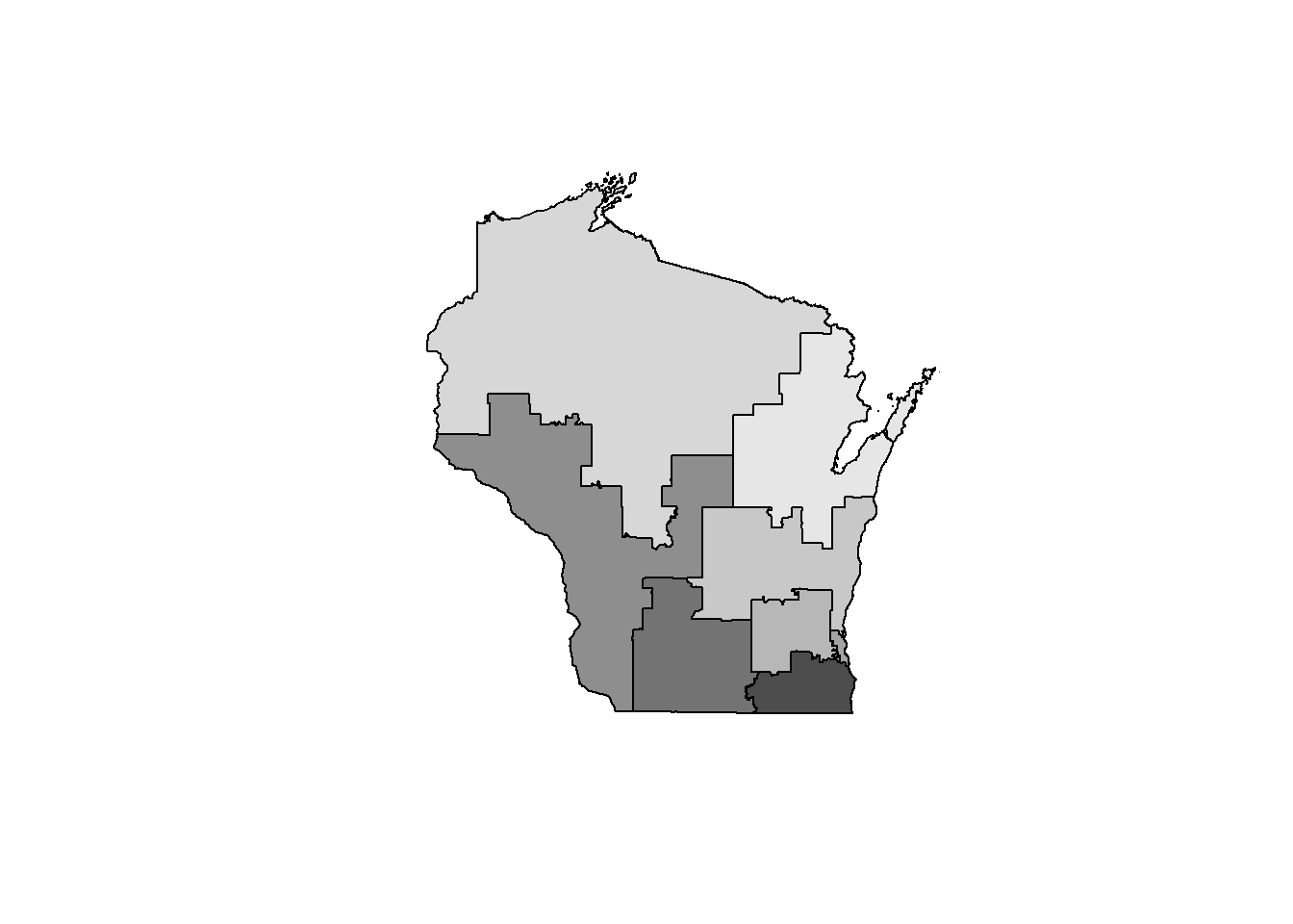
wi_merged <- wi_shp |>
  st_transform(4326) |>
  inner_join(wi_results, by = c("DISTRICT" = "district"))
head(wi_merged, width = Inf)
Simple feature collection with 6 features and 23 fields
Geometry type: MULTIPOLYGON
Dimension: XY
Bounding box: xmin: -92.808 ymin: 42.49198 xmax: -87.50719 ymax: 45.20957
Geodetic CRS: WGS 84
STATENAME ID DISTRICT STARTCONG ENDCONG DISTRICTSI COUNTY PAGE LAW
1 Wisconsin 055113114001 1 113 114 <NA> <NA> <NA> <NA>
2 Wisconsin 055113114002 2 113 114 <NA> <NA> <NA> <NA>
3 Wisconsin 055113114003 3 113 114 <NA> <NA> <NA> <NA>
4 Wisconsin 055113114004 4 113 114 <NA> <NA> <NA> <NA>
5 Wisconsin 055113114005 5 113 114 <NA> <NA> <NA> <NA>
6 Wisconsin 055113114006 6 113 114 <NA> <NA> <NA> <NA>
NOTE BESTDEC FINALNOTE RNOTE LASTCHANGE
1 <NA> <NA> {"From US Census website"} <NA> 2016-05-29 16:44:10.857626
2 <NA> <NA> {"From US Census website"} <NA> 2016-05-29 16:44:10.857626
3 <NA> <NA> {"From US Census website"} <NA> 2016-05-29 16:44:10.857626
4 <NA> <NA> {"From US Census website"} <NA> 2016-05-29 16:44:10.857626
5 <NA> <NA> {"From US Census website"} <NA> 2016-05-29 16:44:10.857626
6 <NA> <NA> {"From US Census website"} <NA> 2016-05-29 16:44:10.857626
FROMCOUNTY state N total_votes d_votes r_votes other_votes r_prop
1 F WI 7 353990 107003 230072 16915 0.6499393
2 F WI 2 397581 273537 124044 0 0.3119968
3 F WI 2 257401 257401 0 0 0.0000000
4 F WI 4 285858 220181 0 65677 0.0000000
5 F WI 3 390507 114477 260706 15324 0.6676090
6 F WI 4 356935 133072 204147 19716 0.5719445
winner geometry
1 Republican MULTIPOLYGON (((-89.08072 4...
2 Democrat MULTIPOLYGON (((-90.43 43.1...
3 Democrat MULTIPOLYGON (((-91.3984 44...
4 Democrat MULTIPOLYGON (((-88.06601 4...
5 Republican MULTIPOLYGON (((-89.01359 4...
6 Republican MULTIPOLYGON (((-89.78555 4...# Color based on winning party
# Note that geom_sf is part of ggplot2 package, while st_geometry is
# part of sf package
wi <- ggplot(data = wi_merged, aes(fill = winner)) +
annotation_map_tile(zoom = 6, type = "osm", progress = "none") +
geom_sf(alpha = 0.5) +
scale_fill_manual("Winning Party", values = c("blue", "red")) +
geom_sf_label(aes(label = DISTRICT), fill = "white") +
theme_void() +
labs(title = "Winners of Wisconsin's Eight Congressional Districts cir. 2016")
wiWarning in st_point_on_surface.sfc(sf::st_zm(x)): st_point_on_surface may not
give correct results for longitude/latitude dataLoading required namespace: raster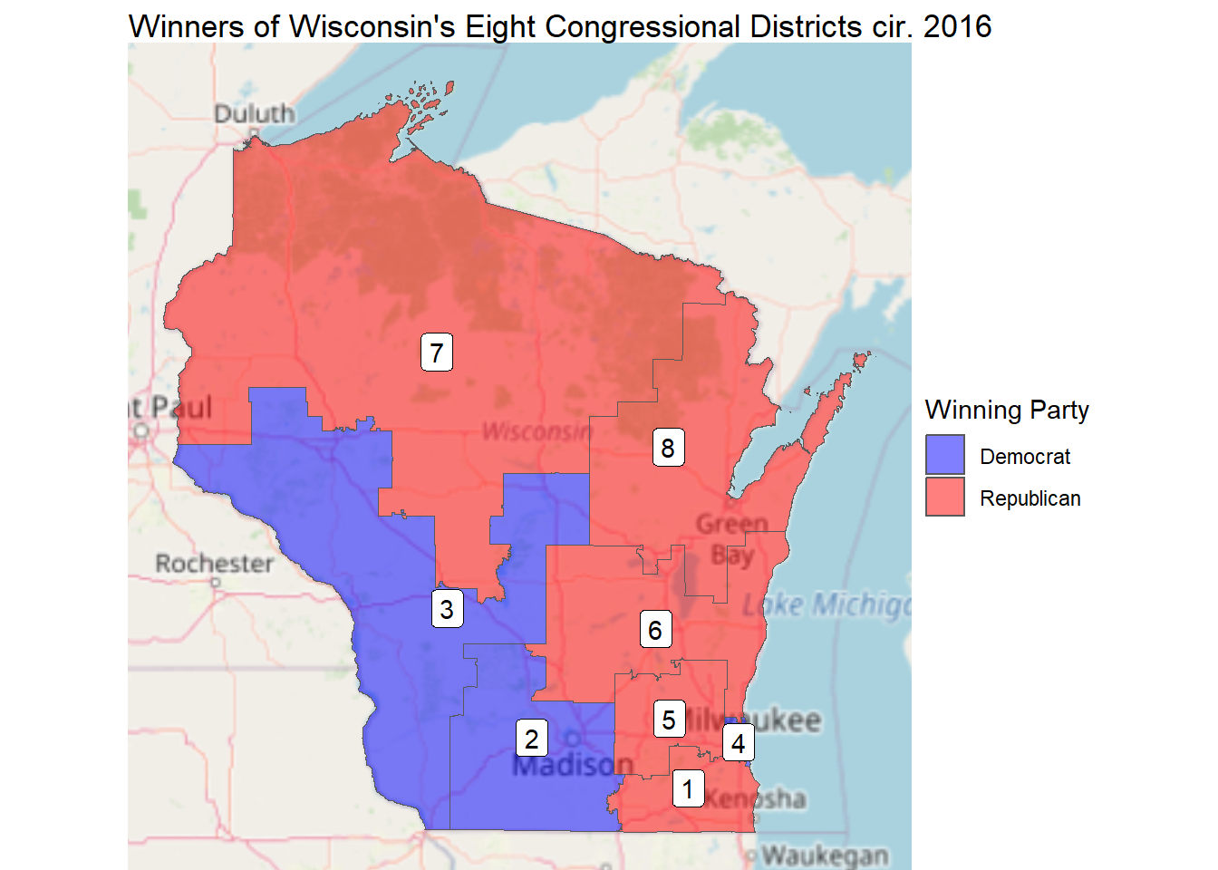
# Color based on proportion Rep.  Be sure to let limits so centered at 0.5.
# This is a choropleth map, where meaningful shading relates to some attribute
wi +
  aes(fill = r_prop) +
  scale_fill_distiller(
    "Proportion\nRepublican",
    palette = "RdBu",
    limits = c(0, 1)
  )
Scale for fill is already present.
Adding another scale for fill, which will replace the existing scale.Warning in st_point_on_surface.sfc(sf::st_zm(x)): st_point_on_surface may not
give correct results for longitude/latitude data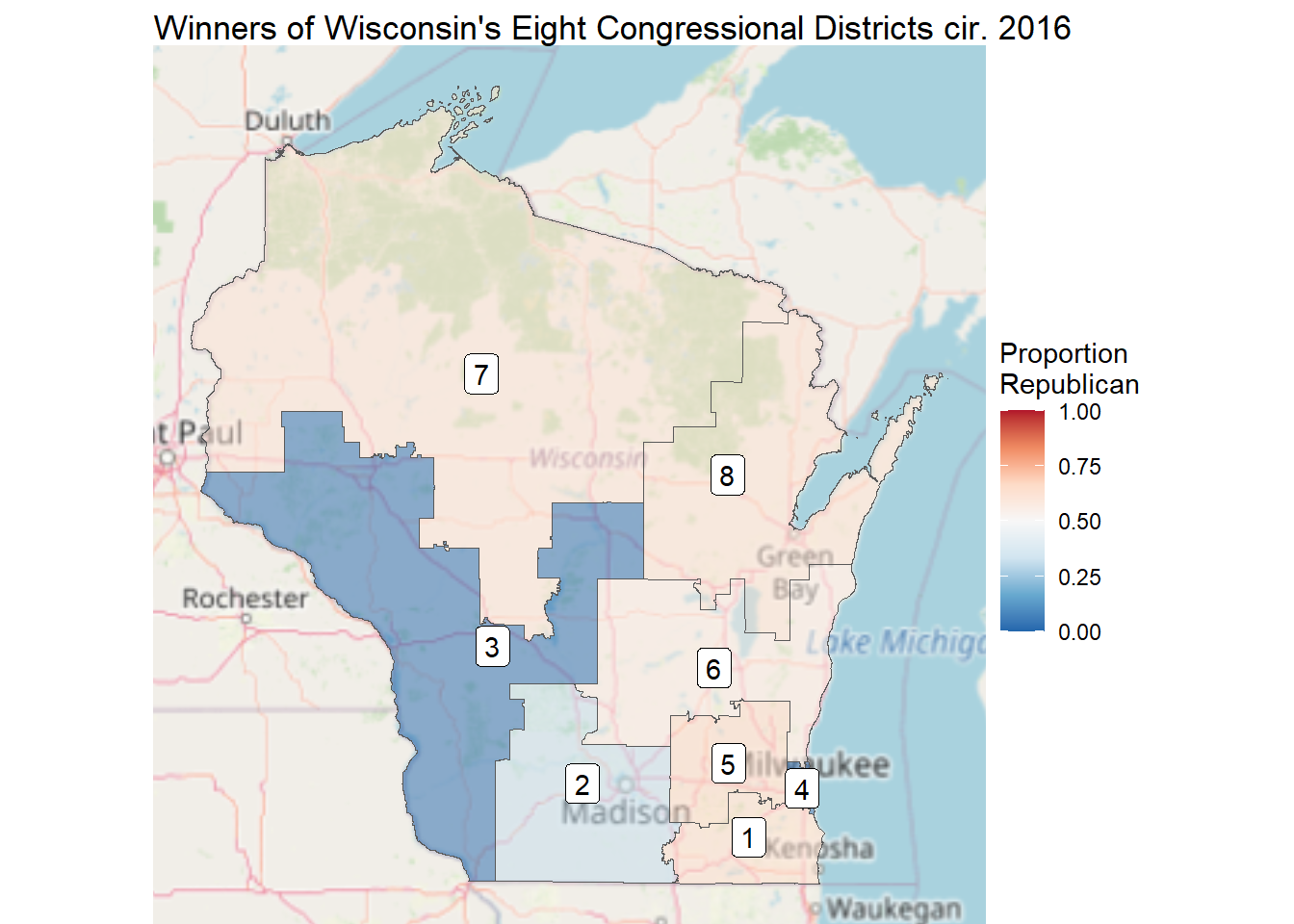
From this map, we can see that quite a few districts (like 2, 3, and 4) definitely contain a strong democratic population, while the districts that are more in the middle (like 1, 7 and 8) are just ever so slightly right leaning. For a party wanting to gerrymander, you would need to group all your opponent’s voters in a select few borders so that their votes go towards an overwhelming victory in those areas, while yours are spread around so that you use your total voters strategically, just barely pulling off a win. With this map, I can definitely understand the argument that Republicans have lopsided control of the state, since it seems like what few Democratic victories there are have very little Republican pushback.