Simulation

# Initial packages required
library(tidyverse)
library(ggplot2)
library(dplyr)
library(mdsr)

Background

Imagine we have new experimental technology to rid Minnesota of springtime snowstorms. Our team of researchers conducts an experiment using this new device over randomly selected areas of Northfield, and compares it with the other half that did not receive any treatment.

Let’s say that this device really works and the weather has a significant decrease in snowfall for the affected areas. Despite this however, it might not always be clear to our researchers that our test had a significant effect. By chance, we could randomly collect a set of measurements from each group that doesn’t demonstrate a difference seen outside the realm of likelihood.

If we carried this test out a good number of times, we would hope to find a statistically low p-value a large proportion of the time. In other words, we would want our test’s power to be large enough so that we can reasonably expect our sample to provide data that correctly rejects the null hypothesis.

Testing for Power

Lets say our researchers collect 20 samples from each group and decide to compare the means of each. Assuming our anti-snow prototype made a genuine difference of 2 less centimeters than the normal amount of snowfall, what is the chance we’ll detect this difference with our sample size? Is our sample size large enough for a majority of the time?

#Finding the proportion of time null is correctly rejected 
set.seed(123)
n1 <- 20
mean1 <- 15
sd1 <- 2.5

n2 <- 20
mean2 <- 13
sd2 <- 2.5

numsims <- 10000


is_sig <- vector("logical", numsims)
for(i in 1:numsims) {
  samp1 <- rnorm(n1, mean1, sd1)
  samp2 <- rnorm(n2, mean2, sd2)
  
  p_value <- t.test(x = samp1, y = samp2)$p.value
  is_sig[i] <- p_value < .05
}

mean(is_sig) #mean is 0.6897

[1] 0.6897

After running our scenario 10,000 times, we end up with a proportion of around .7 for iterations where we reject the null hypothesis. While it might seem like 70% of the time is not great and we should want our value as close to 100% as possible, it’s important to keep in mind that simulations like these are conducted as precursors for real world studies with real world restrictions. Our unfortunate researchers don’t have an unlimited budget and would prefer not to expend resources once our test is past a reasonable success rate.

The National Institute of Health says, “Sufficient sample size should be maintained to obtain … a power as high as 0.8 or 0.9”. Additionally, even if a power value lies below this threshold, we can’t necessarily conclude the study as ineffective. Striving for a “cost-effective sample size” that minimizes the price and duration could be different from one project to the next. For the purposes of this example however, assume our team is looking to meet a power greater than or equal .8 while

numsims = 1000
power <- vector("double", 30)
sampsize <- vector("double", 30)
for (j in 1:30){
  n1 <- 2 * j
  n2 <- n1
  is_sig <- vector("logical", numsims)
  
  
for(i in 1:numsims) {
  samp1 <- rnorm(n1, mean1, sd1)
  samp2 <- rnorm(n2, mean2, sd2)
  
  p_value <- t.test(x = samp1, y = samp2)$p.value
  is_sig[i] <- p_value < .05
}
  
  
  power[j] <- mean(is_sig)
  #print(power[j])
  #print(j*2)
  sampsize[j] <- n1
}

tibble(n_per_group = sampsize, pow = power) |>
  ggplot(aes(x = n_per_group, y = pow)) +
  geom_line() +
  geom_hline(yintercept = .8, color = "red")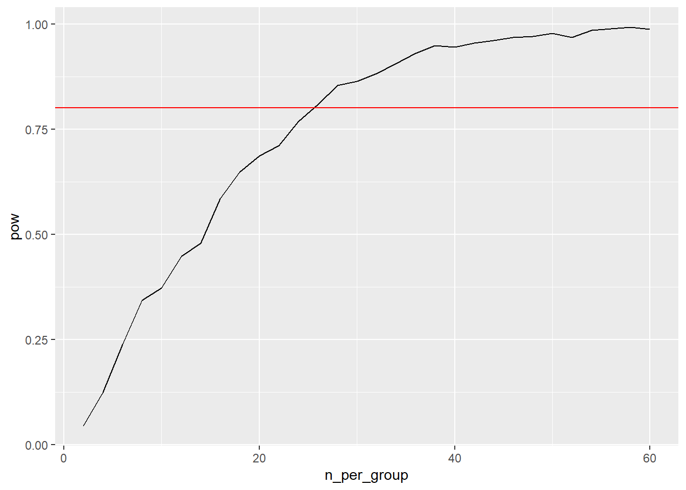

Our graph suggests a sample size of 26 is sufficient for this study, as this is the first value for n that pushes our power past the .8 benchmark. We can also see diminishing returns as our value for n increases with how the graph’s growth slows down more and more.

However, this is assuming that our real difference between means is 2 centimeters and our standard deviations for both distributions is 2.5 cm. The real world distributions may not necessarily follow the specifications we’ve established in our artificial world. Let’s conduct this simulation so that it covers potential differences between means.

Power Curves

Let’s say we expect with reasonable certainty that our treatment group’s mean is within 3 centimeters from the expected normal mean. We can run a simulation to show what amounts per sample group are sufficient.

set.seed(123)
numsims = 1000
pow_tib <- tibble(
   n_per_group = numeric(), 
   pow = numeric(), 
   iteration = numeric()
)


min_n <- tibble(
  xcoord = numeric(),
  ycoord = numeric(), 
  iteration = numeric()
)

for (a in 1:6){
  diff <- a*.5
  mean2 <- mean1 - diff
  power <- vector("double", 30)
  sampsize <- vector("double", 30)
  new <- TRUE
  
for (j in 1:30){
  n1 <- 2 * j
  n2 <- n1
  is_sig <- vector("logical", numsims)
  
  
for(i in 1:numsims) {
  samp1 <- rnorm(n1, mean1, sd1)
  samp2 <- rnorm(n2, mean2, sd2)
  
  p_value <- t.test(x = samp1, y = samp2)$p.value
  is_sig[i] <- p_value < .05
}
  
  
  power[j] <- mean(is_sig)
  #print(j*2)
  sampsize[j] <- n1
  
  if (new==TRUE & power[j] > .8){
    min_n <- min_n |>
      add_row(xcoord = sampsize[j], ycoord = power[j], iteration = diff)
    new<-FALSE
    #label1 <- c(label1, sampsize[j])
  }
  
}
  pow_tib <- pow_tib |>
    add_row(n_per_group = sampsize, pow = power, iteration = diff)

}
pow_tib <- pow_tib |>
  full_join(min_n) 

pow_tib$iteration<-as.factor(pow_tib$iteration)
pow_tib |>
  ggplot() +
  geom_line(aes(x = n_per_group, y = pow, color = iteration), linewidth = 1.1) +
  geom_hline(yintercept = .8, color = "red") + 
  geom_point(aes(x = xcoord, y = ycoord)) +
  geom_text(
    aes(x = xcoord, y = ycoord, label=xcoord),
    nudge_x=0.2, nudge_y=0.03,
    check_overlap=T) +
  labs(color = "Difference Between Means", x = "Number of Samples per Group", y = "Power", title = "Power Curves for Anti-Snow Prototype Testing", subtitle = "Red line represents power of .8") +
  theme_mdsr()

In light of plots like these, let’s make a function that allows us to create power graphs for potential means now (note that this now assumes our standard deviations are consistent between the two groups).

pow_mean <- function(true_mean, mean_list, sd1, numsims){
  set.seed(123)
  sd2 <- sd1
numsims = 2000
pow_tib <- tibble(
   n_per_group = numeric(), 
   pow = numeric(), 
   iteration = numeric()
)

min_n <- tibble(
  xcoord = numeric(),
  ycoord = numeric(), 
  iteration = numeric()
)

for (a in mean_list){
  mean1 <- true_mean
  mean2 <- a
  power <- vector("double", 30)
  sampsize <- vector("double", 30)
  new <- TRUE
  
for (j in 1:30){
  n1 <- 2 * j
  n2 <- n1
  is_sig <- vector("logical", numsims)
  
  
for(i in 1:numsims) {
  samp1 <- rnorm(n1, mean1, sd1)
  samp2 <- rnorm(n2, mean2, sd2)
  
  p_value <- t.test(x = samp1, y = samp2)$p.value
  is_sig[i] <- p_value < .05
}
  
  
  power[j] <- mean(is_sig)
  #print(power[j])
  #print(j*2)
  sampsize[j] <- n1
  
  if (new==TRUE & power[j] > .8){
    min_n <- min_n |>
      add_row(xcoord = sampsize[j], ycoord = power[j], iteration = a)
    new<-FALSE
    #label1 <- c(label1, sampsize[j])
  }
  
}
  pow_tib <- pow_tib |>
    add_row(n_per_group = sampsize, pow = power, iteration = a)

}
pow_tib <- pow_tib |>
  full_join(min_n) 

pow_tib$iteration<-as.factor(pow_tib$iteration)
pow_tib |>
  ggplot() +
  geom_line(aes(x = n_per_group, y = pow, color = iteration), linewidth = 1.1) +
  geom_hline(yintercept = .8, color = "red") + 
  geom_point(aes(x = xcoord, y = ycoord)) +
  geom_text(
    aes(x = xcoord, y = ycoord, label=xcoord),
    nudge_x=0.2, nudge_y=0.03,
    check_overlap=T) +
  labs(color = "Test Group Mean (cm)", x = "Number of Samples per Group", y = "Power", title = "Power Curves for Anti-Snow Prototype Testing", subtitle = "Red line represents power of .8") +
  theme_mdsr()
}

This function works essentially the same way our previous chunk did, but now we can manually input the potential mean values we want to test. We do this by passing a list of our means as an argument, and iterating through this list for our outer-most for loop, and computing a t-test on normal distributions following our specifications.

Now let’s test our function:

my_means <- c(12.5, 13, 16.5, 16.9, 16.3)
pow_mean(15, my_means, 2.5, 1000)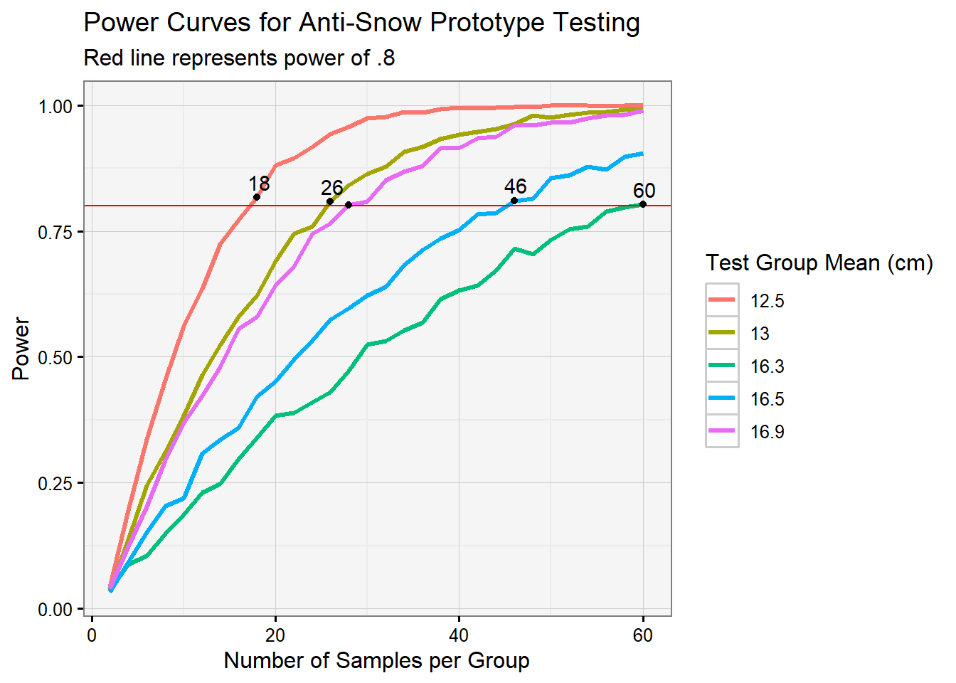

Something interesting to note is that 13cm and 16.9cm have nearly identical curves, which makes sense from the fact that their distances from 15 are nearly equal.

Overall, the mean values in our list that were closer to our original mean of 15 had a tougher time reaching a power of .8 proportion. What’s interesting is that 16.3 cm resulted in 60 samples needed just to barely hit this threshold, while a mean of 12.5 cm hit .8 decently early and even makes it to a proportion of 1 later on.

This makes sense because the less of a difference between our distributions, the more overlap they’ll share, and our samples would reflect this. Having a difference of only 1.3 cm in snowfall in our simulation implies that the researchers will have to commit more effort and resources into the collection of data. This highlights an interesting trade-off: either our anti-snow device performs its job well and allows for an less intensive gathering process, or it makes only a slight difference in snowfall and our surveyors have to pick up the slack to uncover this.

For the beginning stages of our research while we’re still trying to develop an effective technology, it may be wise to put more resources into gathering larger samples since slight improvements being uncovered could point that we’re headed in the right direction. That being said, we often wouldn’t want to expend so much money during an uncertain period of testing. However, with simulations like these, we can be reasonably confident that our tests would uncover a real difference if one did exist, it’s only a matter of how hard should we look for it.